


Next: Suggested Modification to Filter
Up: Verifying the Correct Simulation
Previous: Results
In this section, further evidence that a factor of  has been neglected will be presented. Graphs obtained using the simulation package Mathematica will be shown which affirm the conjecture that equation (2.2) has a factor missing.
Figure 8.23:
Plots of H(s) and HA(s)
 |
The top plot in figure 8.23 shows plots of the transfer function as a cascade of pole zero pairs, HA(s), given by equation (2.1),
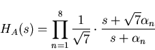
where  and
and 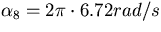 .
.
The bottom plot of the same figure is a plot of the function H(s) which HA(s) purports to approximate. H(s) is given by equation (2.2)
![\begin{displaymath}
H_{A}(s)\approx \frac{ \sqrt{2 \pi f_0}}{s^{\frac{1}{2}}} \q...
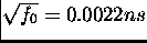
...ere} f_{0}=\frac{\alpha_{1}}{2 \pi \sqrt[4]{7}}\approx 5\mu Hz.\end{displaymath}](img316.gif)
If it is actually the case that
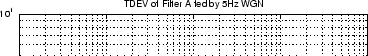
then it would be expected that a log-log plot of each would result in curves with gradients of  where
where
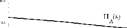
Referring again to the top plot figure 8.23, it can be seen that HA(s) approximates  behaviour as it has approximately the same gradient as the bottom plot. But HA(s) is displaced upwards from H(s). By considering the vertical intercepts it may be seen, for example, that
so  . This suggests that a factor of is required in order that
  , as before.
Next: Suggested Modification to Filter
Up: Verifying the Correct Simulation
Previous: Results
Mark J Ivens
11/13/1997