One Possible Interpretation of the ETSI Noise Model

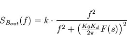
 In this section the results from 5.1 and 5.2 will be compared to show one possible interpretation of the ETSI noise model. The above equation (5.13) can be put into the form

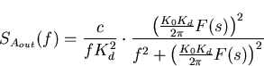$$S_{A_{out}}(f)=\frac{c}{fK_d^2} \cdot \frac{\left(\frac{K_0 ... ... F(s)\right)^2}{f^2 + \left(\frac{K_0K_d}{2 \pi} F(s)\right)^2}$$ (41)

and by comparing it with (5.7)

$$S_{out_{f}}(f)=\frac{\sigma^2}{2B_n} K_f^2 \frac{f_0}{f}\frac{B^2}{f^2 + B^2}$$

it is evident that the model has assumed that

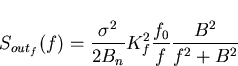
A similar analysis involving (5.10) and (5.12) yields

$$S_{B_{out}}(f)= k \cdot \frac{f^2}{f^2+\left(\frac{K_0 K_d}{2 \pi}F(s)\right)^2}$$ (42)

which by comparison with (5.8), namely

$$S_{out_{w}}(f)=\frac{\sigma^2}{2B_n} K_w^2\frac{f^2}{f^2 + B^2}$$

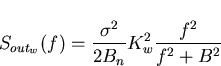
leads to the same correspondence (5.15), (5.16) between the ETSI and PLL models as before and the additional relation  

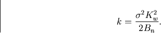$$k=\frac{\sigma^2K_w^2}{2B_n}.$$ (43)

If F(s)=1, as assumed, a first-order loop is obtained. For a first order loop, the 3-dB bandwidth (3.16) after [11] is

$$K=K_0 K_d \mathrm{[rad/sec]}$$

in radians/sec. In Hz this is

$$K=\frac{K_0 K_d}{2 \pi}\mathrm{[Hz]}$$ (44)

Hence the ETSI noise model can be thought of as simulating the noise produced by a 1st order PLL of bandwidth $B=\frac{K_0 K_d}{2\pi}$Hz.