


Next: Problems with the SEC
Up: Theoretical Analysis of the
Previous: Comparison with Published Approximations
In this section the form of the masks for the wander of a clock in locked mode presented in section 2.3 will be predicted. This will be done by making reference to the asymptotic behaviour of approximations to the TDEV of the noise generated at the output of the ETSI noise model. By referring to table 4.1 reprinted below this will allow the noise sources dominant at particular observation intervals to be approximately found.
Table 6.1:
Reproduction of table 4.1 showing TDEV behaviour when presented with various sources of noise
| Noise Process |
Slope of  |
| White Phase Modulation |
 |
| Flicker Phase Modulation |
 |
| White Frequency Modulation |
 |
| Flicker Frequency Modulation |
 |
| Random Walk Frequency Modulation |
 |
Consider once again the expressions for the TDEV produced by the two branches of the ETSI noise model, equations (6.1) and (6.2) reprinted below.
Limiting values in agreement with other published results have already been obtained ![[*]](/~mivens/icons.gif/foot_motif.gif) .
From the form of the above equations, it is evident that (6.13) the bottom equation is dominant for small and (6.12) is dominant at large .So it can be seen that
.
From the form of the above equations, it is evident that (6.13) the bottom equation is dominant for small and (6.12) is dominant at large .So it can be seen that 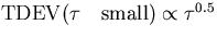 which from table 4.1 is indicative of white phase noise.
Since from equation (6.4)
which from table 4.1 is indicative of white phase noise.
Since from equation (6.4)
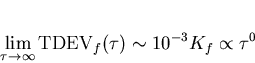
it is expected that flat TDEV is exhibited at large observation intervals at a level of 10-3 Kf ns.
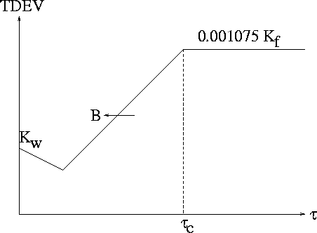
The TDEV behaviour at intermediate observation intervals will now be discussed. Equations (6.12) and (6.13) may be put in the form
By considering the form of the above two equations behaviour it is expected that at shorter observation intervals (6.15) will initiate dominate with (6.14) becoming more significant as increases until the curve exhibits strong flicker frequency ( ) behaviour. As
  it is expected that flat TDEV flicker phase noise dominates.
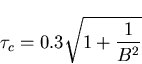
An approximation for the top of the beginning of the flat flicker phase behaviour as shown in diagram 6.1 has also been obtained [4], [14].
it is expected that flat TDEV flicker phase noise dominates.
An approximation for the top of the beginning of the flat flicker phase behaviour as shown in diagram 6.1 has also been obtained [4], [14].
|  |
(56) |
Figure 6.1:
Illustration of asymptotic expressions obtained
 |
Next: Problems with the SEC
Up: Theoretical Analysis of the
Previous: Comparison with Published Approximations
Mark J Ivens
11/13/1997