One argument as to the non-convergence of typical noise sources is the following which has been adapted from one presented by Telecoms Solutions Ltd [24]. It runs as follows. Consider a physical clock being measured or some real-time simulation being performed. In both cases a necessarily finite number of samples N of the time error are collected at regular intervals ![]() over an observation period
over an observation period ![]() . From signal theory, the lowest possible frequency that can be resolved by such a set is
. From signal theory, the lowest possible frequency that can be resolved by such a set is ![]() . Therefore if data were collected over a longer observation time, lower frequencies would contribute to a standard deviation being calculated. For a gaussian distributed noise source which has a power spectral density that is independent of frequency, this simply improves the reliability of the statistical measure. But for a noise source whose frequency power spectrum varies as
. Therefore if data were collected over a longer observation time, lower frequencies would contribute to a standard deviation being calculated. For a gaussian distributed noise source which has a power spectral density that is independent of frequency, this simply improves the reliability of the statistical measure. But for a noise source whose frequency power spectrum varies as ![]() , the standard deviation will grow as the number of points increases. The issue is therefore to obtain a statistical measure that will converge as record length increases otherwise nothing may be measured that makes any sense.
, the standard deviation will grow as the number of points increases. The issue is therefore to obtain a statistical measure that will converge as record length increases otherwise nothing may be measured that makes any sense.
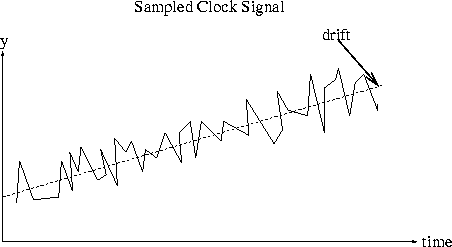
Consider a noise signal with a strong low frequency component. This low frequency component may be thought of as a drift. If one considers the diagram in figure 4.1, one can see that an average over the first half of the curve would be different to one computed over the second half. Thus the average and therefore the variance would not converge.
It is reported [22] that this divergence can readily be seen if one notes that by using Pareseval's theorem, the classical variance of some time series with symmetrical two-sided spectral density ![]() can be written
can be written
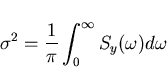 |
(25) |